Pima Indian Diabetes – It's just me

Yesterday I posted an example of the Pima dataset which provide data on the features of an individual and their likelihood to be diabetic. I didn’t get great results (only 67%), so I wanted to take another look and see if there was anything that I could change to make it better. The dataset is pretty small, only 768 records. In my readings, it showed that when you have a small population of data you can use K-Fold Cross Validation to improve the performance of the model.

K-Fold splits the data into k folds or groups. For instance if you set k to be 3, the data will be split into 1 validation set and 2 training sets. For each k the 2 training sets will be used for… fitting the model and the remaining will be used for validation. SciKitLearn has a KFold objects that you can use to parcel the data into the sets. An interesting point that I didn’t catch at first is that the split function returns sets of indices, not a new list of data.

for train_index, test_index in kf.split(x_data,y_data):

So now that we have our data split into groups, we need to loop over those groups to train the model. Remembering that the split data is just an array of indices, we need to populate our training and test data.

    X_train, X_test = x_data[train_index], x_data[test_index]
    y_train, y_split_test = y_data[train_index], y_data[test_index]

Just like the previous Pima example, we build, compile, fit and evaluate our model.

    model = models.Sequential()
    model.add(layers.Dense(16, activation='relu', input_shape=(8,)))
    model.add(layers.Dense(16, activation='relu'))
    model.add(layers.Dense(1, activation='sigmoid'))

    model.compile(optimizer='rmsprop', loss='binary_crossentropy',
                metrics=['accuracy'])

    history = model.fit(X_train, y_train, epochs=epochs, batch_size=15  )
    results = model.evaluate(X_test, y_split_test)

Now to capture the metrics of each fold, we need to store them in an array and I set aside the model with the best performance.

    current = results[1]
    m = 0
    if(len(accuracy_per_fold) > 0):
        m = max(accuracy_per_fold)
 
    if current > m :
        best_model = model
        chosen_model = pass_index

    loss_per_fold.append(results[0])
    accuracy_per_fold.append(results[1])

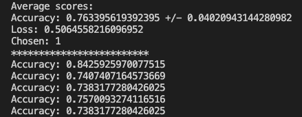
Putting it all together after all folds have been processed, we can print the results.

Now we can run our test data through the model and check out the results.

y_new = best_model.predict_classes(x_test) 
total = len(y_new)
correct = 0
for i in range(len(accuracy_per_fold)):
    print(f'Accuracy: {accuracy_per_fold[i]}')

for i in range(len(x_test)): 
    if y_test[i] == y_new[i]:
        correct +=1

print(correct / total)

Everything worked and based on the randomized test data I was able to achieve a 75% accuracy where the previous method yielded 67%. The full code can be found on GitHub. Just like the other posts, these are just my learnings from the book Deep Learning with Python from Francois Chollet. If any expert reads through this and there is something that I missed or was found to be incorrect, please drop a comment. I am learning so any correction would be appreciated.

I wanted to take another look at binary classifications and see if I could use what I learned on the Pima Indian data set. This is a data set that describes some features of a population and then we try to predict whether someone will have diabetes. The shape of the data is (769,9) and the 9 columns are:

Pregnancies
Glucose
Blood Pressure
Skin Thickness
Insulin
BMI
Diabetes Pedigree Function
Age
Outcome

These are the features that we have to work with. This data is in csv, so the columns are actually a string so we will need to convert that. Let’s load the data and convert it to a numpy array and do the conversion to float32.

with open('pima_indian_diabetes.csv', newline='') as csvfile:
    dataset = list(csv.reader(csvfile))

data = np.array(dataset)
data = data[1:]
data = data.astype('float32')

Obviously, this assumes that the file is in the same directory as your Python file. Originally I used the pandas read_csv, but it returns a DataFrame so it was failing to do the extractions that you will see in a minute. This took me longer than I care to mention before I figured out why it was failing to slice. Just like the IMDB example, we need to separate the features from the outcome.

# 8 features and 1 outcome columns
X = data[:, 0:8]
Y = data[:, 8:]

Now that we have our data separated, we need to split out the training and test data with scikit’s train_test_split. I will choose a 70/30 split.

x_train, x_test, y_train, y_test = model_selection.train_test_split(
    X, Y, train_size=0.7, test_size=0.3, random_state=42)

Now we have to define our model, which is an interesting section. I am using the same model as the IMDB data, but we have some options. We have to change the shape for the input since we only have 8 features (IMDB has 10000). We also need to define the neurons on each level based on the inputs. I will set it to 16, but it must be at least the size of the input which is 8. I get different results when I change this around which I will share.

model = models.Sequential()
model.add(layers.Dense(16, activation='relu', input_shape=(8,)))
model.add(layers.Dense(16, activation='relu'))
model.add(layers.Dense(1, activation='sigmoid'))

Again we use RMS Prop and Binary Cross Entropy and track the accuracy metrics. We also split out our training data and validation data.

model.compile(optimizer='rmsprop', loss='binary_crossentropy',
              metrics=['accuracy'])

x_val = x_train[:350]
partial_x_train = x_train[350:]

y_val = y_train[:350]
partial_y_train = y_train[350:]

Now we can apply the data to the model and see the results. I chose 40 epochs, but we will test different iterations. We will also adjust the number of hidden units.

history = model.fit(partial_x_train, partial_y_train, epochs=40,
                    batch_size=1, validation_data=(x_val, y_val))

If we look at the loss graph with 40 epochs and 16 hidden units, the graph seems to track nicely. Our accuracy seems to level of for a while and the climbs a little higher.

What happens if we add more hidden units, let’s say 32. The loss and accuracy is not as smooth. The accuracy is higher, but it could be overfitting the training data. I should mention that the batch size is 15.

For the last test, I want to put the hidden units back to 16, but run more epochs: 100. We can see that the performance doesn’t change that much, but the accuracy does something strange. The only thing I can think is that there is a lot of overfitting

You might get different results due to the random sampling. The prediction results were not what I was hoping for, so there will be some more experimentation needed. Maybe I will drop some columns and see how the model performs. To get the charts you can use matplotlib.

history_dict = history.history

loss_values = history_dict['loss']
val_loss_values = history_dict['val_loss']

accuracy_values = history_dict['accuracy']
val_accuracy_values = history_dict['val_accuracy']

epochs = range(1, epochs+1)

plt.plot(epochs, loss_values, 'bo', label='Training Loss')
plt.plot(epochs, val_loss_values, 'b', label='Validation Loss')

plt.title('Training and Validation Loss')
plt.xlabel('Epochs')
plt.ylabel('Loss')
plt.legend()
plt.show()


plt.plot(epochs, accuracy_values, 'bo', label='Training Accuracy')
plt.plot(epochs, val_accuracy_values, 'b', label='Validation Accuracy')

plt.title('Training and Validation Accuracy')
plt.xlabel('Epochs')
plt.ylabel('Loss')
plt.legend()
plt.show()

The full code can be found on github. In summary, this is just playing around with some data and running some experiments with adjusting the hyperparameters. It would be great if someone with more experience in machine learning would add some comments and highlight my mistakes or maybe some improvements.

Tag: Pima Indian Diabetes

K-Fold and Pima

ML – A Novice Series (Pima Indians)