Recently while reworking our app to add multi-language support I came across the need to use the intl api outside of the component structures. I tried a couple of different paths, such as a singleton-like provider that is populated by a wrapper component when it is mounted. This worked fine, but was really ugly.
For my use case I have the need to load the language file (data) from the server at runtime, so we needed a way to dynamically load the intl provider after the fact. I didn’t find a way to do that, so we will have to make sure that the data is available when the components at the root are mounted (not a big deal). What I did find, however, was in their api I can create a new instance of the intl object outside of the provider.
There are some considerations with having two instances of the intl object floating around like memory usage, but for our user load that isn’t really an issue for us. To build this out we need to supply a two character locale string, so for that I am using the package locale2. I don’t think anyone could have made that package any easier to use. Like I mentioned, I needed to load the language data from the server when the page is rendered. To extract the language data, I use simple function to pull it from the window object. Now that I have all that I need, I can create the new intl object and return that as an export.
If you are doing multiple languages in React, then this is the tool you want to use. Here is a quick tutorial on how to use it.
Since you want to allow multiple language everywhere in the app, they have create a wrapper control so that the api is available everywhere.
import { IntlProvider } from 'react-intl'
This library works off of json files that have the key/value pairs that give an id to the text that you want to show. Here is an example of the file that will be required.
You can see that it is a simple json file with only one level. The key is what you will use later to retrieve the text that you want. You will create a new json for each new language that you want to support. You will conditionally load that file based on the language. Now that we have a language file, let use the IntlProvider.
Now that we have set up our provider with a file, we can move on to using the provider api. There are a couple of ways to use their api, as a higher order component or as a hook. I using functional components so naturally I use the hooks.
There are many methods in the intl object, but the one that I am going to show here is formatMessage. formatMessage takes a object with one property: id.
{
   id: 'app.get_started_button.title'
}
The id can be anything you want, but I tend to create a dot separated string based on where the text exists in the app. To wrap it up, all you need to do is pass this object to the formatMessage method.
That’s it. Now when you add new language files, you can load them conditionally and pass them to the provider. If you have questions, feel free to reach out to me on Twitter @hivie7510 or email me.
For the second time in a year I need a package to create an ICalendar (*.ics) file in my projects. I tried a couple different packages, but they either didn’t work well or they did not have what I needed requiring me to modify it. I decided that I needed to just build one from the standard. I also have never published a package to the npm registry, so I figured it was time to do both. You can checkout the Github here.
For my immediate needs I required the ability to create an event or a collection of events. These come in the form of a VCalendar and a VEvent. I started googling to find the references for the standards. I came across ICalendar.org which seemed to have most of what I was looking for, but I found it hard to digest in the HTML format, so I decided to go straight to the RFC linked above.
I Started with a simple folder structure. The names are self-describing.
I wanted to follow a builder pattern and have the creation be fluid. This means that the builder is returned in each call so that you can chain the method calls. I like the way it looks and I think it is easier to read.
I wanted to make sure that I didn’t have to polyfill so I used the current version of js which is while you will see classes instead of functional objects. Both of the CalendarBuilder and the EventBuilder are almost the same, they have a constructor, build method, validation method and then the setter methods. Here is an example of the CalendarBuilder.
In the standard there are some supporting objects like an Attendee and Organizer so I have objects for those. Currently I am using the uuid package to generate the required uid field. I may look for another implementation because it is pretty large, but it is ok for now.
In the end, it is pretty simple to execute to get the ics text that you can use in a file or send to a download (if hosted on the web).
const {
    CalendarBuilder,
    EventBuilder,
    Attendee,
    Organizer,
    Role,
    CalendarUserType,
    RSVPType
} = require('ics-standard-compliant-file-generator')

/*

    To import the package you will need to either run this example outside of the root
    or modify temporarily the package.json to change the name.  Otherwise, the package
    will not install because there will be a name conflict

*/

/*

    Start with creating a Calendar Builder, this does not need to happen at first but it is logical to start here
    The Calendar Builder is the container and the actual generator of the *.ics file

*/
var c = new CalendarBuilder()
c.setUrl('http://www.mycalendar.com')
c.setSource('http://www.mycalendar.com/test.ics')
c.setColor('red')
c.addCategory('Meeting')
c.addCategories('my meeting, you meeting')
c.setName('HOME')

/*

    Now lets build a single event by instantiating an Event Builder
    We can create the bare minimum required for an event

*/
var eb = new EventBuilder()
eb.addOrganizer(new Organizer('testOrganizer@gmail.com', 'Test Organizer'))
    .addAttendee(
        new Attendee(
            'testAttendee@gmail.com',
            'Test Attendee',
            null,
            'test-delegate-from@test.com',
            'test-delegate-to@test.com',
            null,
            'test-sent-by@test.com',
            Role.CHAIR,
            CalendarUserType.INDIVIDUAL,
            RSVPType.TRUE
        )
    )
    .setStart(new Date(2021, 0, 1, 20, 00))
    .setEnd(new Date(2021, 0, 2, 20, 00))
    .setSummary('Party Time')
    .setDescription("We're having a pool party")

//Now that we have described our event, we can add it to the Calendar Builder
c.addEventBuilder(eb)

//All that is left is to call the build the file contents
let icsContent = c.build()

//At this point you use which ever method you want to use to create the file
//For testing I just pushed the console output to a file
console.log(icsContent)

//The call from the terminal then becomes:
// node index.js > test.ics
After running this, you will get an output similar to this:
I am still working on this, because I want to add more validation and add the other calendar objects that are compatible such as the VTodo and VJournal.
In my draft posts, I have a ton of notes on how I setup the nano, but none of it works. I have probably spent upwards of 10 hours trying to get it running. The main issue that I have is trying to get OpenCV to install correctly.
There were so many resources on the web that had different approaches, and just like my experience few of them worked for even fewer people. There was a script from someone at NVidia which downloaded, unzipped and did a few other things, but it didn’t compile.
I think I know why that script didn’t work. The last thing the script does is run cmake to generate the make file. Not my area of expertise, but it is not generating the makefile. I tried even barebones cmake .. but still nothing more than the CMakefiles folder. Honestly, I have no idea what I am doing, so I have going to wipe the drive and start over. I hope I can get that done tonight, but time will tell. I will have a step by step post once I figure this thing out.
As I was going through the chapter on convnets in Chollet’s book, Deep Learning with Python, one of the things that I found interesting was the ability to extend an existing trained model. When you think about image recognition, I can’t imagine being able to collect enough images to be able to build a decent model. I thought about an application that could track soccer players on the field and detect how often they were engaged with the ball. Engagement would be defined as the amount of time they were spotted within 1 to 2 meters of the ball.
I think this would be an interesting project, but collecting images of all of the angles that players might find themselves in would be a challenge if not impossible. I wonder how many images of each player would it take to train the model. One of the things that might work is using data augmentation or more specifically taking the same images and mutate them into new images. The mutation could be a translation or an offset in the frame to make the image different, at least to the machine. These images would add to the existing pool and improve the model since there is now more training data. Keras takes care of those mutations with their ImageDataGenerator class.
Convolution using a windowed view of the image and moves that image around to find local features. In contrast, Dense layers look at the whole of the features to train. I am an not an artist so I won’t try to show an example of a convolution window, but think of reading the news paper through a magnifying glass and moving it around until eventually you have covered the whole page.
Chollet gives an explanation of strides and padding, which seem straightforward. I think the best explanation from another well known site MachineLearningMastery. The purpose of the padding is really to give each pixel the change the be in the center of the window. Since the window move 1 pixel at a time from left to right, unless the size of this image is large enough, it is impossible to center the border pixels. For a 5 X 5 image and a 3 X 3 window, it will be impossible to center each pixel, but it you add that image such that it is a 7 X 7 dimensioned image, you can center the pixels.
I am going to post the code from the book since it is more concise, but you can get the true source from Chollet’s GitHub. This code assumes that you have downloaded the cats vs dogs dataset from Kaggle and you have loaded the data and separated them out. I have posted my version on GitHub, but again it is derived from the authors code.
#We need to setup the environment and some paths to our images:
import os
import shutil
from keras import layers
from keras import models
from keras import optimizers
from keras.preprocessing.image import ImageDataGenerator
os.environ['KMP_DUPLICATE_LIB_OK']='True'

base_dir = '/Users/heathivie/Downloads/cats_and_dogs_small'
train_dir = os.path.join(base_dir, 'train')
validation_dir = os.path.join(base_dir, 'validation')
test_dir = os.path.join(base_dir, 'test')
I needed to add this piece os.environ[‘KMP_DUPLICATE_LIB_OK’]=’True’ because it was failing with this error:
OMP: Error #15: Initializing libiomp5.dylib, but found libiomp5.dylib already initialized.
OMP: Hint: This means that multiple copies of the OpenMP runtime have been linked into the program. That is dangerous, since it can degrade performance or cause incorrect results. The best thing to do is to ensure that only a single OpenMP runtime is linked into the process, e.g. by avoiding static linking of the OpenMP runtime in any library. As an unsafe, unsupported, undocumented workaround you can set the environment variable KMP_DUPLICATE_LIB_OK=TRUE to allow the program to continue to execute, but that may cause crashes or silently produce incorrect results. For more information, please see http://www.intel.com/software/products/support/
There are a ton of images that need to be processed and used for training, so we will need to use Keras’ ImageDataGenerator. It is a python generator that looks through the files and yields the image as it is available. Here we will load the data for training.
The first train_datagen is filled with parameters to support the data augmentation. The next to pieces there simple setup the path, target (image size) and batch size. It also specifies what the class model is and since we are doing a classification of two types (cats & dogs) we will use binary.
Like the earlier posts we will still be using a Sequential model, but we will start with the ConvD layers.
Above we have specified that we want to have a 3 X 3 window, 32 filters (channels), relu as our activation and the image shape of 150 X 150 X 3. One thing to note, we need to do a classification which requires a Dense layer to process, so how do we translate a 3D tensor to fit the dense layer. Keras gives a Flatten method to do this. It final shape is a 1D tensor (X * Y * Channel).
We finalize it with a single Dense layer with the sigmoid activation. The last piece is to compile the model. For this we will use the loss function binary_crossentropy since this is a classification problem with 2 possible outcomes.We will again use the optimizer RMS prop, but here we will specify a learning rate or the rate at which it moves when doing the gradient. Lastly, we configure it to return the accuracy metrics.
Now we can run the fit method, supplying it with the training and validation generators that we created above. The step* parameters are there to make sure that our generators don’t run forever. This is configured to run 30 epochs at 100 steps each, so on my machine this takes about 10 minutes. Make sure you save your model.
history = model.fit(
    train_generator,
    steps_per_epoch=100,
    epochs=30,
    validation_data=validation_generator,
    validation_steps=50)

model.save('ch_5_cat_dogs.h5')
After running through all of the epoch’s, I achieved a 0.75 accuracy. This is what it looked like:
After you have saved your model, you can go a take picture of your cat or dog (or grab one of the internet) and use it to predict whether it is a cat or a dog.
import os
import numpy
from keras.models import load_model
from keras.preprocessing import image
base_dir = '/Users/heathivie/Downloads/cats_and_dogs_small'
# load model
model = load_model('ch_5_cat_dogs.h5')
# summarize model.
model.summary()
file = test_dir = os.path.join(base_dir, 'test/cats/download.jpeg')
f = image.load_img(file, target_size=(150, 150, 3))
x = image.img_to_array(f)
# the first param is the batch size

y = x.reshape((1, 150, 150, 3)).astype('float32')

classes = model.predict_classes(y)
print(classes)
I used this image of my amazing dog Fergus and the prediction was correct, he was indeed a dog.
The next post I will do is use a pre-training convnet, which I think it awesome. I am going to continue talking about the goal of a model that can detect someone and their proximity to a ball.
Yesterday I posted an example of the Pima dataset which provide data on the features of an individual and their likelihood to be diabetic. I didn’t get great results (only 67%), so I wanted to take another look and see if there was anything that I could change to make it better. The dataset is pretty small, only 768 records. In my readings, it showed that when you have a small population of data you can use K-Fold Cross Validation to improve the performance of the model.
K-Fold splits the data into k folds or groups. For instance if you set k to be 3, the data will be split into 1 validation set and 2 training sets. For each k the 2 training sets will be used for… fitting the model and the remaining will be used for validation. SciKitLearn has a KFold objects that you can use to parcel the data into the sets. An interesting point that I didn’t catch at first is that the split function returns sets of indices, not a new list of data.
for train_index, test_index in kf.split(x_data,y_data):
So now that we have our data split into groups, we need to loop over those groups to train the model. Remembering that the split data is just an array of indices, we need to populate our training and test data.
Now to capture the metrics of each fold, we need to store them in an array and I set aside the model with the best performance.
    current = results[1]
    m = 0
    if(len(accuracy_per_fold) > 0):
        m = max(accuracy_per_fold)

    if current > m :
        best_model = model
        chosen_model = pass_index

    loss_per_fold.append(results[0])
    accuracy_per_fold.append(results[1])
Putting it all together after all folds have been processed, we can print the results.
Now we can run our test data through the model and check out the results.
y_new = best_model.predict_classes(x_test)
total = len(y_new)
correct = 0
for i in range(len(accuracy_per_fold)):
    print(f'Accuracy: {accuracy_per_fold[i]}')

for i in range(len(x_test)):
    if y_test[i] == y_new[i]:
        correct +=1

print(correct / total)
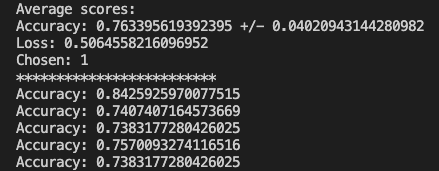
Everything worked and based on the randomized test data I was able to achieve a 75% accuracy where the previous method yielded 67%. The full code can be found on GitHub. Just like the other posts, these are just my learnings from the book Deep Learning with Python from Francois Chollet. If any expert reads through this and there is something that I missed or was found to be incorrect, please drop a comment. I am learning so any correction would be appreciated.
I wanted to take another look at binary classifications and see if I could use what I learned on the Pima Indian data set. This is a data set that describes some features of a population and then we try to predict whether someone will have diabetes. The shape of the data is (769,9) and the 9 columns are:
Pregnancies
Glucose
Blood Pressure
Skin Thickness
Insulin
BMI
Diabetes Pedigree Function
Age
Outcome
These are the features that we have to work with. This data is in csv, so the columns are actually a string so we will need to convert that. Let’s load the data and convert it to a numpy array and do the conversion to float32.
with open('pima_indian_diabetes.csv', newline='') as csvfile:
    dataset = list(csv.reader(csvfile))

data = np.array(dataset)
data = data[1:]
data = data.astype('float32')
Obviously, this assumes that the file is in the same directory as your Python file. Originally I used the pandas read_csv, but it returns a DataFrame so it was failing to do the extractions that you will see in a minute. This took me longer than I care to mention before I figured out why it was failing to slice. Just like the IMDB example, we need to separate the features from the outcome.
# 8 features and 1 outcome columns
X = data[:, 0:8]
Y = data[:, 8:]
Now that we have our data separated, we need to split out the training and test data with scikit’s train_test_split. I will choose a 70/30 split.
Now we have to define our model, which is an interesting section. I am using the same model as the IMDB data, but we have some options. We have to change the shape for the input since we only have 8 features (IMDB has 10000). We also need to define the neurons on each level based on the inputs. I will set it to 16, but it must be at least the size of the input which is 8. I get different results when I change this around which I will share.
model = models.Sequential()
model.add(layers.Dense(16, activation='relu', input_shape=(8,)))
model.add(layers.Dense(16, activation='relu'))
model.add(layers.Dense(1, activation='sigmoid'))
Again we use RMS Prop and Binary Cross Entropy and track the accuracy metrics. We also split out our training data and validation data.
Now we can apply the data to the model and see the results. I chose 40 epochs, but we will test different iterations. We will also adjust the number of hidden units.
history = model.fit(partial_x_train, partial_y_train, epochs=40,
                    batch_size=1, validation_data=(x_val, y_val))
If we look at the loss graph with 40 epochs and 16 hidden units, the graph seems to track nicely. Our accuracy seems to level of for a while and the climbs a little higher.
What happens if we add more hidden units, let’s say 32. The loss and accuracy is not as smooth. The accuracy is higher, but it could be overfitting the training data. I should mention that the batch size is 15.
For the last test, I want to put the hidden units back to 16, but run more epochs: 100. We can see that the performance doesn’t change that much, but the accuracy does something strange. The only thing I can think is that there is a lot of overfitting
You might get different results due to the random sampling. The prediction results were not what I was hoping for, so there will be some more experimentation needed. Maybe I will drop some columns and see how the model performs. To get the charts you can use matplotlib.
The full code can be found on github. In summary, this is just playing around with some data and running some experiments with adjusting the hyperparameters. It would be great if someone with more experience in machine learning would add some comments and highlight my mistakes or maybe some improvements.
For the last couple of weeks, I have been trying to learn more about machine learning. The obvious path was to soak up as much as I could from various blog posts, but I wasn’t getting everything that I needed. I bought this book by Joel Grus Data Science from Scratch. It was really good and gave me a great introduction into the concepts and terms. I read that front to back and read some chapters many (many) times. I felt like I was off to a good start, but I felt like I needed more textbook style content. Deep Learning with Python turned out to be that book.
Deep Learning with Python turned is a book from 2018 by Francois Chollet, the creator of Keras. As I am going through the chapters, I am going to post here about what I understood about the text and an example if possible.
I watched a PluralSight video on ML and it talked about a google site called Colab. I had been using Kaggle, but I think Colab has more power. The first thing I noticed on Colab was the code completion. This tool was built for engineers so I should not have been surprised, they really did a great job. Did I mention that it is free, you only need a Google account.
Moving on. Disclaimer: I may make mistakes or omit pertinent concepts, but I am learning at the same time. After going over Tensors and what they are, the books jumps into a classification problem. This is a binary classification because it is reviewing reviews from IMDB to determine if the are positive or negative. Since there is only two states (positive/negative), this is defined as a binary classification. Another cool thing about Keras is that it comes with datasets for you to experiment with.
Starting with the IMDB import, you can extract out your training and testing datasets.
The load_dataset call takes an integer which specifies, like it name says, the number of frequent words that you want to load. I think it is obvious that the data is broken into training and testing sets. What might not be obvious is why the data and label are stored as a pair. If you think about a the basic linear equation, you have y= mx + b. In this case, you are given the x and the y (Data/Label) and you need to solve for the m and b. Thinking back to algebra we remember that m is equal to the slope of the line and b is the offset. We need to find the m and b to make the question correct. This is what the neural network will do. You will give it an equation and it will solve for the remaining variables and it will even adjust the m and b until it gets to a certain level of accuracy. Word soup.
Again, now that we have our training and test data partitioned we can start to see how we can use it to train the machine to predict if a review is positive or negative. Since a network can only take a number and more specifically a tensor, we need to change the words to a vector. There is a lot of information between where we are now and where we want to be, so I will just show how we do that.
def vectorize_sequences(sequences, dimension = 10000):
  results = np.zeros((len(sequences),dimension))
  for i, sequence in enumerate(sequences):
    results[i,sequence] = 1
  return results
This creates a tensor of 10000 entries and sets them all to zero. Then it loops over all of the data in the training data and sets the cell to 1 where the word is present in the sequence. The sequence is simply a list filled with the indices of the position of the words. Now that we can turn our individual lists into a tensor we can convert our training and test data to a collection of these tensors:
Our data is now prepared and ready to go, so we need to configure our network. There is a key concept here that needs to be understood, activation function. The activation function is what determines whether the output of the neuron is 0 or 1. There are many different types of activation functions, but in this example he used the Rectified Linear Unit (relu) function. You can check out the link for more information.
Since a neural network consists of the input, output and one ore more hidden layers, we will need to do that configuration.
#We have to make sure that import the model and layer objects
from keras import models
from keras import layers

model = models.Sequential()
model.add(layers.Dense(16, activation='relu',input_shape = (10000,)))
model.add(layers.Dense(16, activation='relu'))
model.add(layers.Dense(1, activation='sigmoid'))
Ok, we have set up the model. Let’s break it down. Since we are working in layers, we define this model to be sequential. Then we configure two hidden layers that will be 16 dimensions which my understanding is that there will be 16 neurons, could be wrong. We also define the shape of the input data, which is our 10,000 element wide tensor. Lastly, since this is a binary classification we will only have a single output.
Before we need to send our training data through the model, we need to compile it. We will compile it to use the RMS Prop optimizer function and the loss function of Binary Cross Entropy. These work well for classification problems. The last parameter will allow us to get some data in the form of history as the machine runs through its trials.
Now we are ready to train the machine! We need to define how many iterations it will attempt to train and the batch size. We also submit the validation data.
history = model.fit(partial_x_train, partial_y_train, epochs=5, batch_size=512, validation_data=(x_val, y_val))
Executing this command will start the machine to learn that given an input X, the model predicts Y. As it loops over, you should see an output like:
When I ran through this example, each time I received different values and this is because of the random sampling. The only thing left is to test out our machine and see how it performs on the test data.
You can see that some are good and some are terrible. I guess that makes sense since so much of what people right cannot be simply distilled down to positive or negative, but this is still impressive. The words in the post are mine and not copied from any other source, but all credit goes to Francois Chollet. Now this was a simple binary classification, the next on is a multiple classification problem where the answer can be 1 of 46 different classes. Here is the colab. Anyways, I will do more reading and report back. The full code is also on github.
For the last several weeks, I have been trying to learn more about data science. I have always enjoyed writing queries for reporting to dig into the stories that the data can tel. Data science takes that interest to a whole new level.
As a typical engineer I haven’t exercised my linear algebra or calculus since my undergraduate. The book (Data Science from Scratch: First Principles with Python 2nd Edition) that I am reading starts hard and fast in that direction. Luckily I have most of my old school books, so I have been speed reading through them to try to reclaim some level of understanding. So I have been a nerd with my stats, linear algebra and calculus books for the last several weeks. Reading them a decade later gives me a new appreciation for the material.
All of that leads to why I am really interested into learning data science. On a project that I am working on there is an opportunity to utilize some machine learning techniques. More specifically, the project asks a sequence of questions to a user to arrive at a customer satisfaction score.
One of the areas that we may be able to employ such techniques is determining the next question (excluding next questions only). It would seem reasonable to have the ability to craft the sequence of questions (let’s call it a survey) based on the answers to the previous ones. If you have n surveys completed, then you might be able to do some multiple regression analysis. This could tell you what the probability of the next question being answer in a certain way. This would allow you to remove questions that you know have a high likelihood of being unnecessary since they are consistently answered the same.
One of the first thing that comes to mind with that approach is there may be some questions that are more important thereby requiring a user’s answer. In other words, they may have more weight and should be removed from the possible exclusion set. Another top of mind concern is the actual ordering of the questions. If the ordering is random such that the questions are independent, how could you predict what the next question is going should not be or does the machine determine the order itself.
I think having the machine determine the order of the questions would be pretty awesome. Would that somehow invalidate the comparison between surveys based on some psychological factors that the order would create, I am not sure. Theoretically, if the questions are truly independent, you should be able to present them in any order. I do believe that they could tell a different story even with the same answers if presented in different ways. ¯\_(ツ)_/¯
So at this point, we have multiple regression to determine what the likely next sequence of questions will be answered in a certain way. This would need to be a multi-pass operation, since you should be checking each successive question to determine if it needs to be asked. It is possible that you could reach a point where no further questions are required.
That now covers the exclusion , but what about including new questions dynamically. Would you have a pool of questions that are related to a product or service to be used for possible inclusion? In that scenario would you only include some static questions and allow machine to add questions from a pool based on prior responses? That seems like a simple decision tree, but given that we are already excluding some questions it seems unreasonable to construct that tree. You could always have a parent-child relationship where one answer prompts a series of new questions, but again that would need to be preordained.
It seems that dynamic inclusion is a much more challenging endeavor. I think I will leave it here for now so I can marinate a little more on this topic.
Recently I have been working on a clinical trial application and needed a way to export all of the data. The client wants the questions to be displayed horizontally, but the data is stored vertically. This is the structure of the data:
Pretty simple schema, the issue is here. This is what they want it to look like:
At first this was a little intimidating, because there are different types of questions in separate tables that would need to be combined and then transposed together. I decided to use the PIVOT function. Now there was an another requirement that needed to be addressed, the columns had to be sorted. This took a little bit of data massaging to get it in the correct pre-pivot format.
To set the stage I have a number of pre-processing steps that I won’t show here, but just know that those steps result in temp table #data. Now that I have all of the data in place, I need to order the questions so that they pivot correctly:
-- PRE-PIVOT PROCESSING
SELECT
    [CaseId] ,
    [Title],
    [Value]
INTO #ordered
FROM #data
ORDER BY
    [CaseId],
    [Title]
Here comes the interesting part. I need to extract all of the columns into a comma delimited string for use in the pivot. For this I need a VARCHAR to hold the delimited fields. Now I can take the data from the #ordered table and generate the fields:
DECLARE @ColumnName AS NVARCHAR(MAX)

SELECT @ColumnName= ISNULL(@ColumnName + ',','')
       + QUOTENAME([Title])
FROM (SELECT DISTINCT [Title]  FROM #ordered ) AS c ORDER BY [Title]
There is another function in there that I didn’t know about before I needed to do this: QUOTENAME. This will take the string and wrap it in square brackets. This allows for strings with spaces to be used for a column name. At this point, we have the @ColumnName variable set with a delimited set of question titles.
Now that we have our columns set, we need to generate the sql that will be executed. For this we need to get the data. We will take use a CTE to collect the data with the new list of columns and pump that into the PIVOT function. The PIVOT function take the aggregate that you want applied to the value field and the column that you want to PIVOT, in my case the @ColumnName array. Lastly, I need to have the rows grouped by the unique CaseId. In the end it looks like this:
DECLARE @query NVARCHAR(MAX);

SET @query = ';WITH p ([CaseId],'+ @ColumnName +') as (SELECT [CaseId],' + @ColumnName + ' from
(
    SELECT
        [CaseId],
        [Title],
        [Value]
    FROM
        #ordered
) x PIVOT (MAX([Value]) for [Title] in ('+@ColumnName+')) p  GROUP BY [CaseId],'+@ColumnName+') SELECT * FROM p '
EXECUTE (@query);
When we execute these queries, we end up with the result that we want:
One note, these values above are strings in the data, so an aggregate does not make sense, so you can use the MAX function to get the exact value.